SageMath GSoC 2018 Projects

We're happy to announce our list of Google Summer of Code projects for 2018! Thank you to everyone involved, all students, mentors and of course, Google! 


Sai Harsh Tondomker (David Coudert and Dima Pasechnik):

Addition of SPQR-tree to graph module

In this project, our goal is to extend the graph theory library in Sage by implementing functionality to find triconnected subgraphs, which will partition an undirected graph into 3-connected components and the construction of the corresponding SPQR-tree. These modules can later be used as pre-processing for several graph problems such as Hamiltonian Cycle, traveling salesman problem.



Meghana M Reddy (David Coudert and Dima Pasechnik):

Addition of SPQR-trees to the graph module of Sage Math

The aim of the project is to code the linear time algorithm for partitioning a graph into 3-connected components and constructing the corresponding SPQR-tree of the graph. Further, this algorithm can be used as a subroutine for several other graph problems such as recognition of chordless graphs, hamiltonian cycle etc.



Filip Ion (Johan Rosenkilde):

Databases and bounds of codes

The following proposal detail some possible improvements of the coding theory component of SageMath. We aim to build databases of precomputed bounds and optimal examples of linear codes for each choice of parameters below a maximum range.



Raghukul Raman (Travis Scrimshaw and Benjamin Hutz):

Rational Point on Varieties

This project aims at implementing basic algorithms for finding rational points on varieties. Classically algebraic variety is defined as the set of solutions of polynomial equations over a number field. A rational point of an algebraic variety is a solution of set of equations in the given field (rational field if not mentioned). Much of the number theory can be viewed as the study of rational point of algebraic varieties. Some of the great achievements of number theory amount to determining the rational points on particular curves. For example, Fermat’s last theorem is equivalent to the statement that for an integer n ≥ 3, the only rational point of the curve xn+yn=zn in P2 over Qare the obvious ones. Common variants of these question include determining the set of all points of V(K) of height up to some bound. The aim of this project is to implement some basic rational point finding algorithms (sieving modulo prime and enumeration) and extend these to product_projective_space scheme.



Dario Asprone (Dima Pasechnik)

Checking graph isomorphism using the Weisfeiler-Lehman algorithm

Currently SageMath checks for graph isomorphism through an internal package with a corresponding method, called isomorphic and contained in sage.groups.perm_gps.partn_ref.refinement_graphs. This method, in addition to being quite convoluted and without much documentation about its inner workings, was last updated in a significant manner in 2011.
The project aims at creating a new package which implements an efficient in practice heuristic method to check if two graphs are isomorphic, using one of the members of the Weisfeiler-Lehman (WL) algorithm hierarchy. An attempt was made in the past at the same task (but with a narrower scope, limited to only implementing the second order version of the WL algorithm), but the code was found to contain a bug and was never implemented/removed from the codebase (see Trac #10482).
To the best of my knowledge, this would be the first working open-source implementation of k-WL, for k > 1.

SageMath GSoC 2017 Projects

6 GSoC SageMath Projects

During the past couple of summers, SageMath successfully managed many Google Summer of Code projects. This year we are again happy to have six projects:

Implementing matroid classes and plotting improvements

(Zachary Gershkoff / Stefan van Zwam)

This project seeks to implement several common matroid classes in SageMath, along with algorithms for their display and relevant computations. The graphic matroid class in particular will be implemented with a representative graph with methods for Whitney switching and minor operations. This will be accompanied by improvements to the graph theory library, with methods relevant to matroids enabled to support multigraphs. Other modules for this project include improved plotting of rank 3 matroids to eliminate false colinearities, computation of a matroid's automorphism group using SageMath's group theory libraries, and faster minor testing based on an existing trac ticket.

Expanding the Functionality of Dynamical Systems

(Rebecca Lauren Miller / Paul Fili and Ben Hutz)

As a member of the sage-dynamics community, researchers have compiled a wishlist for algorithms and functionality they would like added. I would like to shorten the wish list for us.For my project I will be completing some desired additions to SAGE from the Sage Dynamics Wiki. I will implement Well’s Algorithm, strengthen the numerical precision in cannonical_height, as well as implement reduced_form for higher dimensions.

Improvement of Complex Dynamics in Sage

(Ben Barros / Adam Towsley and Ben Hutz)

There are three major things that I would like to implement to improve the functionality of Sage in the area Complex Dynamics. The details of the project are summarized in the following list:

• Complex Dynamics Graphical package: Integrate or implement a complex dynamics software such as Mandel into Sage. This will be done by creating an optional package for Sage. If there is enough demand, the package may become a standard package for Sage at some point.

• Spider Algorithm: The object of the Spider Algorithm is to construct polynomials with assigned combinatorics. For example, we may want to find a polynomial that has a periodic orbit of period 7. The Spider Algorithm provides a way for us to compute this polynomial efficiently. I plan to implement this algorithm into Sage.

• Coercion: If you have a map defined over Q, you should be able to take the image of a point over C (i.e. somewhere you have a well-defined embedding) without having to use the command "change_ring()". Something similar works for polynomials in Sage but it does not work for morphisms/schemes.

Linear-time Implementation of Modular Decomposition of Undirected and Directed Graphs

(Lokesh Jain / Dima Pasechnik)

This project is aimed at providing linear time implementation for modular decomposition of graphs and digraphs. Modular decomposition is decomposition of graph into modules. A module is a subset of vertices and it is a generalization of connected component in graph. Let us take for example a module X. For any vertex v ∉ X it is either connected or not connected to every vertex of X. Another property of module is that a module can be subset of another module. There are various algorithms which have been published for modular decomposition of graphs. The focus in this project is on linear time complexity algorithms which can be practically implemented. The project further aims to use the modules developed for modular decomposition to implement other functionality like skew partitions. Skew partition is partition of graph into two sets of vertices such that induced graph formed by one set is disconnected and induced graph formed by other set is complement of the first. Modular decomposition is a very important concept in Graph Theory and it has a number of use cases. For instance it has been an important tool for solving optimization and combinatorics problems.

Modular Decomposition of graphs and digraphs

(Maria Ioanna Spyrakoy / Dima Pasechnik)

Modular decomposition of (di)graphs is a generalization of the concept of the decomposition of (di)graphs into connected components. Its current implementation in Sage relies on badly broken abandoned C code, and badly needs to be replaced by something that works and is not too slow. However, the only open-source implementations of some of these procedures are either in Java or in Perl, and thus aren't really useful for Sage.

Note: A attentive reader might notice the similarity between those projects. They will be split regarding the type of graph and be coordinated to not overlap but to augment each other.

Visualizing constructs in cluster algebras and quiver representations

(Bryan Wang / Travis Scrimshaw)

I aim to implement visualizations of several key constructs in cluster algebras and quiver representations. The first is Auslander-Reiten quivers, for at least the A_n and D_n cases. The second is labelled endomorphism quivers and mutations within a cluster category, focusing on the A_n case. The third is posets of down-mutations for the A_n case. These features will be useful not only for research purposes, but also as nice examples to play around with and learn from. Aside from these features, I am interested in implementing features for the Quantum Cluster Algebras project.

All the best for this summer, thank you to Google for making this possible, and sorry to all those candidates who didn't make it ...

Sage Days 70 - Berkeley - November 2015

+Dennis Stein brought his cameras and tools to Sage Days 70: 

Sage Days 70 - Berkeley - November 2015 from Dennis Stein on Vimeo.

R's sapply in Numpy

One quick blog entry about sapply and numpy:

Usually, sapply is equal to list comprehensions in Python.
i.e. [f(x) for x in range(1, 10)] is sapply(1:10, f).

But: When you want to apply a function (mapping a number to a vector!) to a vector, you get a matrix. R's sapply does raise the rank of the output to two, while in Numpy you have to push the vector to a higher rank via the magical vector[:, np.newaxis].

In [1]: import numpy as np

In [2]: def f(x):
   ...:     return np.array([4,2,3,9.1,-1]) * x
   ...: 

In [3]: f(9)
Out[3]: array([ 36. ,  18. ,  27. ,  81.9,  -9. ])

In [4]: vals = np.linspace(-1,1,20)

In [5]: np.apply_along_axis(f, 1, vals[:, np.newaxis])
Out[5]: 
array([[-4.        , -2.        , -3.        , -9.1       ,  1.        ],
       [-3.57894737, -1.78947368, -2.68421053, -8.14210526,  0.89473684],
       [-3.15789474, -1.57894737, -2.36842105, -7.18421053,  0.78947368],
       [-2.73684211, -1.36842105, -2.05263158, -6.22631579,  0.68421053],
       [-2.31578947, -1.15789474, -1.73684211, -5.26842105,  0.57894737],
       [-1.89473684, -0.94736842, -1.42105263, -4.31052632,  0.47368421],
       [-1.47368421, -0.73684211, -1.10526316, -3.35263158,  0.36842105],
       [-1.05263158, -0.52631579, -0.78947368, -2.39473684,  0.26315789],
       [-0.63157895, -0.31578947, -0.47368421, -1.43684211,  0.15789474],
       [-0.21052632, -0.10526316, -0.15789474, -0.47894737,  0.05263158],
       [ 0.21052632,  0.10526316,  0.15789474,  0.47894737, -0.05263158],
       [ 0.63157895,  0.31578947,  0.47368421,  1.43684211, -0.15789474],
       [ 1.05263158,  0.52631579,  0.78947368,  2.39473684, -0.26315789],
       [ 1.47368421,  0.73684211,  1.10526316,  3.35263158, -0.36842105],
       [ 1.89473684,  0.94736842,  1.42105263,  4.31052632, -0.47368421],
       [ 2.31578947,  1.15789474,  1.73684211,  5.26842105, -0.57894737],
       [ 2.73684211,  1.36842105,  2.05263158,  6.22631579, -0.68421053],
       [ 3.15789474,  1.57894737,  2.36842105,  7.18421053, -0.78947368],
       [ 3.57894737,  1.78947368,  2.68421053,  8.14210526, -0.89473684],
       [ 4.        ,  2.        ,  3.        ,  9.1       , -1.        ]])

It also works happily for an additional argument weights, which will be defined in the variable w.

In [6]: def f(x, weights):
    return weights * x
   ...: 

In [7]: w = np.array([-2,-1,5,1.1])

In [8]: np.apply_along_axis(f, 1, vals[:, np.newaxis], w)
Out[8]: 
array([[ 2.        ,  1.        , -5.        , -1.1       ],
       [ 1.78947368,  0.89473684, -4.47368421, -0.98421053],
       [ 1.57894737,  0.78947368, -3.94736842, -0.86842105],
       [ 1.36842105,  0.68421053, -3.42105263, -0.75263158],
       [ 1.15789474,  0.57894737, -2.89473684, -0.63684211],
       [ 0.94736842,  0.47368421, -2.36842105, -0.52105263],
       [ 0.73684211,  0.36842105, -1.84210526, -0.40526316],
       [ 0.52631579,  0.26315789, -1.31578947, -0.28947368],
       [ 0.31578947,  0.15789474, -0.78947368, -0.17368421],
       [ 0.10526316,  0.05263158, -0.26315789, -0.05789474],
       [-0.10526316, -0.05263158,  0.26315789,  0.05789474],
       [-0.31578947, -0.15789474,  0.78947368,  0.17368421],
       [-0.52631579, -0.26315789,  1.31578947,  0.28947368],
       [-0.73684211, -0.36842105,  1.84210526,  0.40526316],
       [-0.94736842, -0.47368421,  2.36842105,  0.52105263],
       [-1.15789474, -0.57894737,  2.89473684,  0.63684211],
       [-1.36842105, -0.68421053,  3.42105263,  0.75263158],
       [-1.57894737, -0.78947368,  3.94736842,  0.86842105],
       [-1.78947368, -0.89473684,  4.47368421,  0.98421053],
       [-2.        , -1.        ,  5.        ,  1.1       ]])

Convert several IPython Notebooks to one huge PDF

The IPython Notebook is a neat interactive document. It mixes headings, formatted text (markdown), formulas, images/pictures and interactive code. This is very neat for creating well-documented code examples.

To make ordinary publishing possible, nbconvert converts this interactive json-based file format to ordinary static HTML or LaTeX. The nbviewer website is a well known example for such a repository of HTML-notebooks.

Converting to LaTeX is also very handy, because then you can compile them to static PDF files -- e.g. think of a proper report or article.

So far I know, each input document is converted to only one output document. For one of my projects, I wanted to merge a whole bunch of IPython Notebooks to one (very large) PDF document! To achieve this, I've looked into the various *.tplx template file and started to build on top of them two new templates: partial and master. As the names suggest, partial is the template for each partial document, and master is essentially empty, but combines all partial documents in an orderly fashion.

You can see this here: github:haraldschilly/python-fuer-mathematiker

In particular:

• partial.tplx: This removes all the preamble and heading stuff and sets the document class to the wonderful subfiles LaTeX class.
• master.tplx: This template contains the default header definitions (inherited from IPython's base template), adds some tweaks of my own (font family, margins, title, and subfiles master class) and an embedded Python script to magically gather all documents!

How it works: First, all partial IPython Notebook files are converted to LaTeX using the partial template. Then, the master.tplx contains a small embedded Python script, which iterates through all partial LaTeX files. They are named numerically as --chaptername. This script inserts all those subdocuments and if there is an  increments in the major-number, it inserts a \chapter{...} heading.

To orchestrate all this, a usual Makefile checks for dependencies and finally uses latexmk with the --shell-escape switch (which is necessary to run the embedded Python). Works like a charm!

I hope this is helpful for some of you.

Mein Email an den VAP

Habe soeben dies an vap1@aon.at gesendet:

Mit Entsetzen muss ich heute lesen, dass österreichweit eine Blokadeinfrastruktur für Netzzensur errichtet wird. Ihr Mitwirken an diesem Akt der Unmündigmachung aller Österreicher_innen ist eine Skandal. Legen Sie mir bitte dar, welche Gesetze beim bloßen Download exakt verletzt werden und in welcher Relation dies zu der angeprangerten Bundesbürger_innenbevormundung steht. Die alten Wirtschaftsmodelle haben ausgedient und Ihr VAP Verein ist eine reine Interessensvertreung für große, längst überholte internationale Konzerne und im Beamtenschimmel verfilzte österreichische Organisationen. Ich hoffe Sie bekommen in den nächsten Wochen und Monaten reichlich Gegenwind zu spüren. Willkommen im 21-ten Jahrhundert!

In Vollendung,
ein Bundesbürger

PS:

Als Wochenendlektüre empfehle ich den Barbara Streisand Effekt:
https://en.wikipedia.org/wiki/Streisand_effect

Netflix in Ubuntu - part 2347 of \infinity

Today, Netflix started in Austria. Well, I thought, give it a try. Too bad, it's really painful in my Linux box. So, if you also have Ubuntu 14.10:

1. Get Chrome Beta 38 or higher
2. Update libnss3 via running this in your terminal:
   
   for pkg in libnss3_3.17-1ubuntu1_amd64.deb libnss3-nssdb_3.17-1ubuntu1_all.deb libnss3-1d_3.17-1ubuntu1_amd64.deb
   do
      wget http://archive.ubuntu.com/ubuntu/pool/main/n/nss/${pkg}
   doneThen install it:
   
   $ sudo dpkg -i libnss*.deb
3. Install the User-Agent Switcher for Chrome
   In its options (right-click on the icon) you have to add a new entry (besides the "String", nothing else really matters):
   
   
   • Name: Netflix
   • String: Mozilla/5.0 (Windows NT 6.3; Win64; x64) AppleWebKit/537.36 (KHTML, like Gecko) Chrome/38.0.2114.2 Safari/537.36
   • Group: keep it empty
   • Indicator: FLX (for Net-Flix)
   
   After that, set it to be active on netflix.com automatically: On the left, in "Permanent Spoof List"...
4. Restart chrome, ... cross your fingers ... and enjoy.
5. Edit: you also have to set the profile properties in netflix to HTML5 (though, I think it still works without doing anything, because there is no silverlight anyways)

New combinatorial designs in Sage - by Nathann Cohen

This is a guest post by Nathann Cohen. 

---

New combinatorial designs in Sage

Below, these graphs are a decomposition of a $K_{13}$ (i.e. the complete graph on 13 points) into copies of $K_4$. Pick two vertices you like: they appear exactly once together in one of the $K_4$.

The second graph shows a decomposition of a $K_{4,4,4}$ (i.e. the complete multipartite graph on $4\times 3$ points) into copies of $K_3$. Pick two vertices you like from different groups: they appear exactly once together in one of the $K_4$.

Sage has gotten quite good at building such decompositions (a specific kind of combinatorial designs) when they exist. This post is about them.

The first object belongs to a family called Balanced Incomplete Block Designs (or $(n,k)$-BIBD), which are defined as "a collection $\mathcal S$ of sets, all of them with size $k$ (here $k=4$), such that any pair of points of a set $X$ with $|X|=n$ (here $n=13$) appears in exactly one set of $\mathcal S$".

The second belongs to the family of Transversal Designs (or $TD(k,n)$) which have a similar definition: consider a set $X$ containing $k$ groups (here $k=3$) of $n$ vertices (here $n=4$). A collection $\mathcal S$ of sets, each of which contains one point from each group, is a $TD(k,n)$ if any two points from different groups appear together in exactly one set of $\mathcal S$.

The main problem with combinatorial designs is to know where they exist. And that is not obvious. Sage does what it can on about that:

• If you want it to build a $(14,4)$-BIBD, it will tell you that none exists.
• If you want it to build a $(16,4)$-BIBD, it will tell you that one exists.
• If you want it to build a $(51,6)$-BIBD, it will tell you that it just not know if there is one (and nobody knows better at the moment)

Examples here:

sage: designs.balanced_incomplete_block_design(14,4,existence=True)
False
sage: designs.balanced_incomplete_block_design(16,4,existence=True)
True
sage: designs.balanced_incomplete_block_design(51,6,existence=True)
Unknown

For a developer (and design lover), the game consists in teaching Sage how to build all combinatorial designs that appear in some research paper. For BIBD as well as for Transversal Designs, on which a LOT of sweat was spent these last months.

For Transversal designs the game is a bit different, as we know that a $TD(k-1,n)$ exists whenever a $TD(k,n)$ exists. Thus, the game consists in finding the largest integer $k_n$ such that a $TD(k_n,n)$ exists. This game is hardly new, and hardly straightforward: In the Handbook of Combinatorial Designs, one can find the table of such $k$ up to $n=10000$ (see here).

The good thing about Sage is that it does not just claim that such a design exists: it also builds it, and there is no better existence proof than that (it is very very quick to check that a combinatorial design is valid). The other good thing is that there is no common database for such data (the Handbook is not updated/printed every night), and that by teaching Sage all new designs found by researchers we build such a database. And it already contains designs that were not known when the Handbook was printed.

Finally, the other other good thing about Sage is that it will soon be able to tell you where those designs come from. Indeed, the most powerful results in the field of Transversal Designs are of the shape "If there exists a $TD(k_1,n_1)$, and a $TD(k_2,n_2)$, ..., and a $TD(k_c,n_c)$, then you can combine them all to obtain a $TD(k,n)$ with $k=k(k_1,...,k_c)$ and $n=n(n_1,...,n_c)$". And it is never very clear how to inverse these functions: if you want to build a $TD(k,n)$, which integers $k_1,...,k_c,n_1,...,n_c$ should you pick ?

Sage knows. It must know it, in order to build these designs anyway. And you can find that data inside. And soon, we will teach it to give you the bibliographical references of the papers in which you can find the right construction to produce the $TD(k,n)$ that you want. And we will provide the right parameters. And the world will be at peace.

A couple of things before we part:

• Transversal Designs (TD), Orthogonal Arrays (OA), and Mutually Orthogonal Latin Squares (MOLS) are all equivalent objects.
• We write a LOT of Transversal Designs code these days, so expect all this to improve very fast.
• You can learn what Sage knows of combinatorial designs right here.

Finally, there are far too many combinatorial designs for one man to learn. If you love combinatorial designs, come join us: Vincent Delecroix, you, and I have code to write together. And if you know a related mathematical results that Sage ignores, come tell us: we could not have gone so far without the mathematical knowledge of Julian Abel. And Sage does not know everything yet.

Have fuuuuuuuuuuuuuuuuuuun !

Nathann

Blüte des Lebens - Georg Kostron

Musik-kritische Ausführungen im Staccato.

Vorweg: dieser Text wird in Kürze ins Lateinische übersetzt.

"Blüte des Lebens" ist eine stimmgewaltige Kraftkomposition. Ausgetüftelte Klänge begleiten diversiv zusammengetragene Klangschnipsel und garnieren - begleitet durch zeitkritischen Text - den ausgeprägten Hang zum liebevollen Detail. Das Album thematisiert an dessen Höhepunkt das Geschraube und Gedrehen an den Knöpfen der absoluten Machtkontrolle in der zentralen Schaltzentrale. Kurz: der tüftelnde Monarch seines unendlich großen Reichs der Effektkiste ist politisch.

Song 01. Raumschiff Maria

Ein routinierter Klick auf das nach rechts blickende Abspieldreieck, es wummert kurz - Dissonanz - zu leise? - kurzes Quietschen und sofort nach der Landung ist klar: dieses Album ist eingekochter Grüntee statt verdünntem Fruchtsaft. Der 1/4 Beat klopft hart ins Ohr, ist verwirrt ob des Textes und der vorsichtige Mitteleuropäer dreht ab Minute 2:30 sicherheitshalber etwas leiser. Ist das etwas zum Beten?

Song 02. Rostiges Rösslein

Versöhnlicher, Chorgesang, Melodie - zurücklehnen. Aber spätestens das Textfragment "Geld arbeitet - nicht" lässt die untertönig bittere Note anklingen. "Zügellos", "Sporen", "Peitsche" und todesbleiche Reiter mahnen den Hörer.

Song 03. Der kleine Tiger

Katzen möchten im monotonen Alltag eingelullt, sicher in der Box hockend, den Tag absitzen. Textlastiges Crescendo, maximal aufgedrehte Stimmen und songstrukturierte Abwechslung konfrontieren sie. Das Album schafft sich Raum und dehnt ... aus. Inneres Unbehagen, Stress und Unentspannung statt schmeichelnder Wohlfühlklänge.

Song 04. Lick My Face (edit)

Besuch einer altbekannten Zeitgenössin aus der "Sophia I" Phase. Musikalisch geben sich Elektronik, Instrument und die menschliche Mundschallöffnung die Hand. Sie zerren sdich gegeneinander in ihre jeweiligen Ecken, kurz kippt es in eine Ecke, nur um später explosiv zurückzuschnalzen.

Verbraucherhinweis: Spätestens an dieser Stelle wird eine erste Verschnaufpause empfohlen.

Song 05. Alle Welt

Vermeintlich poppig geht es weiter, aber der Refrain bestätigt: dies täuscht. Ein Abgesang auf das kollektive Weltbild. Inzwischen passen die sperrigen Klänge problemlos in den weit aufgemachten Raum. Es knarzt.

Song 06. Knapp vor Schaltraum

Herrlich! Das intellektuell stimulierende Latein dämpft die aufgewühlten animalistischen Emotionen, es trägt, man spürt: das Zentrum kommt für Wahr näher und man steht im Auge des Taifuns. Avantgardistische Elektronik, dann eine Orgel, ganz von der Ferne kanonenschussartige Paukenschläge.

Song 07. Süßes Kind

Fast fließend landet der Hörer in einem Liebeslied? Wer wird hier besungen? Die aufopfernde Schlusssteigerung dreht nochmals schnell am Sinn, erzeugt Verwirrung, die Entspannung ist schnell vorbei und schon ist 08 bereit für die Bühne.

Song 08. Schaltraum (edit)

Bitte Anschnallen. Treibender, hämmernder, minimalistischer Druck. Die Beats tänzeln mit sich selbst im trockenen Vakuum. Ein technokratisch editiertes Interludum entzieht jegliche Humanität, die elektrische Steuerung übernimmt das Ruder. Fast spirituelle Songskizzen beenden diesen Raubzug am Verstand. Wer hat ihn geraubt?

Song 09. Beistrich

Ein versöhnlich-humoristischer Aufgesang an die jugendliche Interpunktionskultur des Web 2.0.

Song 10. Wunderschön (edit)

Hitverdächtige Durtöne, Chöre, Mitsingmelodie, Geige, hin-und-her: heftig illussioniert, warm eingewickelt, was ist da los? Relativierende Schlagwörter gravitieren den Hörer wieder auf den rauhen Betonboden der Realität. Diese Blendung ist eine erfolgreiche.

Song 11. Küss den Tango

Der vielleicht treibendste Song des Albums. Kurzweilige Strukturzerlegungen und eingeworfene Schrägtöne bringen die schon gewohnte Unsicherheit wieder zurück. Auf-und-ab gesungene "Ah"s schrubben die bereits geröteten Großhirnfurchen wieder sauber. Es riecht nach Schweiß und Reinigungsmittel.

Song 12. Hans Tanz

Zurücklehnende Melodien, breit, kaugummiartig. Ein Akkordeon, etwas Echo, und diverse Aufforderungen an Hans verhallen im Hintergrund. Nachdenklichkeit macht sich breit. Ein gänsehautgarantierender Schlusschor.

Song 13. Der A

Nicht die Spur einer Scheu vor der Zahl 13. Es soll einfach weiter-so gehen, halt, ja, einfach weiter ... so. Hilflos gefangen im musikalischen Spinnennetz dieses Albums spannt sich ein weiterer Radialfaden in Richtung klassischem Clubsound. Tanz endlich. Im Kreis. Spätestens seit Snoweden wissen wir, dass sich auch Drohnen ständig im Kreis herum drehen.

Song 14. Tanzboutique

Der letzte Song. Ist Steigerung überhaupt noch möglich? Ein Schrei, Auftakt, 3, 2, 1. Was passiert hier? Ein sauber auskomponierter Song im deutsch-lateinischen Zwiegespräch wirft mit mehrdeutigen Fragmenten um sich. Dem Hörer wird ein kleine geheime Tür gezeigt: es ist der Notausgang in die Wirklichkeit.

Bonustrack.

Wer ein paar Minuten warten kann, wird mit einem acapellaartigem Songfragment belohnt. Es endet offen, ein Vorgeschmack auf einen Teil 2?

Abschlussbeurteilung:

9 von 10 Aes Grave.

Links:

f/undSeinManager

Sage GSoC 2014 Projects

This year, Sage is happy to announce that it will be running five Google Summer of Code projects. Welcome everyone to the Sage community and all the best to your summer filled with exiting projects ;-)

EDIT: lmonade related projects are listed here.

Nikhil Peter Raj (Volker Braun):

Improvements to the Sage Android App

This project aims to improve upon the existing app by improving both internal structure and external user experience, the former by replacing and redoing certain modules of the app (JSON Parsing, HTTP Requests and Exception Handling) and the latter by redesigning the UI so it conforms to the latest standards and specifications of Android Design, as well as adding extra features to the code input such as Syntax Highlighting and options to record and store custom inserts.

Amit Jamadagni (Miguel Angel Marco-Buzunariz)

Knot theory implementation

The project mainly deals with the implementation of various links, knots presentations and calculating various related invariants. The main aim of the project is to achieve: Conversion between different representations of Knots and Links to mention a few: Gauss code to Braid Word, Braid word to DT code, Gauss code to DT code. Implementation of various invariants: Alexander Polynomial, Conway Polynomial. Stiefert Matrix, Jones Polynomial

Jayant Apte (Stefan van Zwam)

Efficient class-specific membership checks, extensions and visualization 

First goal of this proposal is to implement efficient testing of a matroid for membership of various classes and to perform single element extensions of matroids that exploit the knowledge that a given matroid belongs to a certain class, to have lower complexity. We also propose implementation of visualization techniques and an application of matroid theory in form of enumeration of network codes for a multisource network coding problem which is one of the timely problems in information theory.

Simon Spicer (William Stein, Jonathan Bober)

Efficient exact analytic rank computation for elliptic curves in Sage

My project would be to implement functionality in Sage to compute the analytic rank of an elliptic curve exactly modulo standard conjectures, with better scaling than existing analytic rank estimation methods. This would necessitate both writing (significant amounts of) new Python and Cython code, as well as porting existing code into the Sage codebase.

Daniel Bell (Ivan Andrus)

iSage - improving the Sage iOS apps

There are several aspects of the Sage iOS apps that needs to be refreshed, improved or implemented. I propose to develop the ability to interact with several Sage services from the app, as well refresh the user interface for the app.

My first Time-Lapse Experiment

Well, my new camera (Panasonic DMC-GX7) has two features I've never had before: stop-motion and time-lapse. The only difference seems to be: the minimum time between the shots is either 1 second or 1 minute - and if there is an "open end" or a fixed number of pictures.

Searching around online, the most important thing to do is to take the shots in manual mode. The reason is, that you do not want to have this flickering. So well, that's easy to do in manual mode: exposure, aperture, ISO and of course the focus. What I didn't read (or didn't notice), but should have done is to also fix the white-balancing! So, in case you want to try this, set it the white balancing to manual.

One cool thing of doing this in stock motion on my camera is, that it automatically converts the images to a movie. Only for one sequence I had to do it on my computer, because the camera wasn't responsive or I've confused it. So, in case you are on a Ubuntu Linux like I am, here is what to do: First, don't bother with ffmpeg or avconv: they are too old and do not have the flag "-start_image" to set the first number of the counter. This sucks!

So instead: mencoder:
Start by moving all the images in a separate directory, then the "P*.JPG" regex pattern matches all your images in alphabetical order. Easy.

$ mencoder -nosound -ovc lavc -lavcopts vcodec=mpeg4:mbd=2:trell:autoaspect:vqscale=3 -vf scale=1920:1080 -mf type=jpeg:fps=5 'mf://P*.JPG' -o OUTPUT.avi
=> see update below

If you have better ideas for the command-line, please post it. fps=5 is for the number of frames per second. I think the quality should be set higher, but no idea which of the switches does this in a sane way.

Now enjoy these three YouTube videos from Vienna (Parlament and City-Hall):

Update:

There is indeed a much better mencoder setting, using x264:

$ mencoder -nosound 'mf://P*.JPG' -mf fps=10:type=jpeg -ovc x264 -x264encopts preset=slow:tune=animation:crf=20 -vf scale=1440:1080 -o time-lapse.avi

Options (for more, check the manpage)

• fps=10: 10 pix/second. 5 is also ok, 20 if you have really a lot of pics.
• tune=animation: sounds reasonable, there is also "film"
• crf=20: recommended switch for setting the quality, could also be 10 or 20, ...
• -vf scale: that could be something different, depends on what you have. (960x720)

When will Sagemath Cloud hit 100,000 user accounts?

The Sagemath Cloud is an online environment for computational mathematics. Get an account, log in, and your web-browser transforms into almost everything you need to study algebra, calculus, numerics, statistics, number and game theory, (computational aspects of) physics, chemistry and all other quantitative sciences. It's built around all sorts of tools and utilities offered in a proper Linux environment. All files can be shared with collaborators and edited in real-time without stepping on each other's toes. Oh wait, there is also a LaTeX editor: given you know LaTeX, qualitative sciences are also covered ;-)

But beware, this posting will only talk about the very first: accounts. Below, I'll explain how I managed to create this page, the plot below and how I let it update automatically every hour - all done solely by SMC!

SMC accounts over time

Sagemath Cloud is very public about what is happening on its servers. This stats link gives you the raw data for the current overall load of the machines. What I did over the last weeks was the following: Every hour I've downloaded this stats json file, parsed it, accumulated some interesting numbers, and stored the processed data in a CSV file.

I did all this in SMC, because it allows you to run your own crontab files. Cron periodically goes through all kind of files to figure out if there is a job to do. Just enter a magical line in your own crontab file, and the given command is run whenever you tell it to do so. You do not have to be logged in!

In my case, it's like this:
First, edit your crontab file:
$ crontab -e
Then enter this line:
0 * * * * python $HOME/get.py

The $HOME is important, because you have to specify the full path where your script sits. (By the way, if you have to start something when the SMC server reboots, use the @reboot descriptor)

So, what is get.py doing? It uses the wonderful requests Python library to retrieve and parse the stats url and extracts some data. Then it appends a line to a CSV file.

Two minutes later (the crontab line starts with a "2"), another script is called which processes this CSV file. It reads the columns via pandas, properly parses the dates into time-series, and allows me to do all sorts of analysis, transformations and plots with it. For example, the plot shown above overlays the raw time series plot with OLS fits done by statsmodels for selected time ranges (where it looks "flat"). We can see the growth trends clearly! Even more important, so far the growth increases and hence we are watching the exponential growth phase as part of the beginning of the usual logistic growth.

The other plots on this statistics page show aggregated time-series data. For example, the plot for the number of concurrent connections is also increasing and reassures that SMC is scaling well.

Concurrent connections to SMC

On this statistics page, there are also a few "dynamic" fields in the HTML content. This is done by jinja2 in such a way, that the template "stats.tmpl" contains the HTML code and "mustache"-style variables. Jinja2 renders this template with some variables and that's it.

import jinja2 as j2
env = j2.Environment(loader=j2.FileSystemLoader("."))
stats = env.get_template("stats.tmpl")
data = {
        'date' : "%s UTC" % datetime.utcnow(),
        'recent_data' : totals.ix[-24:].to_html()
}
with open("stats.html", "wb") as output:
    output.write(stats.render(**data))

The last step of the script is to actually publish the files to the webserver. That's rather straight forward. First and only once, create ssh keys via ssh-keygen without a password and then use ssh-copy-id -i ~/.ssh/id_dsa.pub name@server to copy over your keys. Subsequent ssh connections will be established without any questions asked, because the remote server knows your identity. I'm using scp to copy the files: scp *.png stats.html name@remote-server:~/target/dir/

Last but not least, when will SMC hit the 100,000 user mark? In less than 6 days the 10,000 mark should be crossed and I hope the trend continues into the upward direction.

Sage announces 3 GSoC projects

Sage is pleased to announce three Google Summer of Code projects for 2013. They focus on speed improvements of symbolic functions, simplifying the distribution and installation procedure on Debian/Linux and ubiquitous accessibility of Sage on the Android platform.

Mathematical Functions Library

Eviatar Bach –  University of British Columbia in Vancouver, Canada

(Mentor: Flavia Stan, Backup: Burcin Erocal)

Sage interfaces with multiple third-party libraries, such as MPFR, GSL, GP/PARI, mpmath, and Maxima, for numerical evaluation of special functions. There are significant discrepancies between these backends in the performance for numerical approximations of the same expression. An initial benchmark reveals, for example, that calculating spherical_bessel_J(1, 5.2) with SciPy is over 100 times faster than with Maxima.

The project has the following goals:

1. develop a benchmark framework to determine which backend should be used by default to evaluate a special function over a specific domain,
2. create symbolic wrappers for all the special functions that can be evaluated numerically by a package included in Sage,
3. create a data structure for generalized hypergeometric functions and extend the symbolic wrappers to obtain representations in terms of generalized hypergeometric functions when possible,
4. implement closure properties for holonomic functions as a next step to improve the symbolic processing of special functions in Sage.

Overall improvement of the Sage Android application

Rasmi Elasmar

(Mentor: Volker Braun, Backup: Harald Schilly)

Although there are already some existing efforts, Sage is still not easily accessible from the Android platform. The Sage Cell client/server infrastructure is an already existing step towards running Sage on a server and communicating back the results. The aim of this proposal is to fix, improve and update the Sage Android application to include new features and functionality, as well as an improved interface for simpler and improved usability. Android's new "Holo" style, sharing of calculations and results, and much more waits to be realized on Android for Sage.

Get Sage ready for Linux distributions

Felix Salfelder – Goethe Universität, Frankfurt, Germany

(Mentor: Tobias Hansen, Julien Puydt, Jeroen Demeyer & John Palmieri )

sage-devel discussion

The aim of this project is to detach the build process of Sage ("the software") from Sage ("the distribution"). The goal is a build system that works within the context of Sage as well as for any GNU/Linux distribution that ships the dependencies for Sage. Distributions that already ship Sage packages or plan to do so are Fedora and Debian. This project is an important step towards making Sage packages in GNU/Linux distributions feasible.


Sage warmly welcomes all three new students and wishes them all the best to learn something new and make an impact in Sage's future developments!

Sage part of Google's Summer of Code 2013

Good News, like last year Sage is once again part of Google's Summer of Code. This means, until April 22 at 19:00 UTC students can submit their applications and mentors will review them and do the matching.

Please share this with prospective students or think about being a mentor this year!

links:

• Sage's GSoC page
• Ideas (check back for updates)

Sage 5.8

Sage 5.8 has been released, download it here.

Also, the documentation page has been updated to reflect the new thematic tutorials. I highly recommend to browse through all those topics to learn more about Sage's ever increasing scope.

Git, Mercurial, Subversion trends

In case you have to convince someone on which horse to bet:

Lenovo x220 Trackpoint and Ubuntu

Although I'm using my Lenovo x220 laptop for more than a year, I discovered the settings for the track-point yesterday (random searches and forums, don't remember). I was never really thinking about it, but the track-point was a bit slow and stiff. The configuration settings of the usual UI configuration menu had no effect at all (yes, certainly a bug), either.

So, to reveal the magic, here it is. I've added a udev configuration file here:

$ cat /etc/udev/rules.d/trackpoint.rules

SUBSYSTEM=="serio", DRIVERS=="psmouse", WAIT_FOR="/sys/devices/platform/i8042/serio1/serio2/sensitivity", ATTR{sensitivity}="240", ATTR{speed}="95", ATTR{press_to_select}="1", ATTR{inertia}="6"


This is just one line for the settings of sensitivity, speed and intertia. You can also play around with them manually, e.g.

$ echo "5" | sudo tee /sys/devices/platform/i8042/serio1/serio2/inertia

Mathematica 9's R integration vs. Rpy2

Some notes about "What's new in Mathematica 9: Builtin R Integration"
To understand what's going on, please open the example: Hierarchical Clustering.

This posting is basically about how to integrate R via Rpy2 in Python and hence also in Sage.

First thing you should notice is the clash of two parallel worlds. MMA's "RSet" command converts and sets the variable y in the scope of R. That's nice, but wouldn't it be much easier, to just have a local variable for that? Second of all, the function definitions inside strings - filled with escaped quotes - is also not that great. Isn't there are better quoting available?

What I want to do is to accomplish something similar with Rpy2. So yes, there are also equivalents to this RSet function, and you can also evaluate arbitrary R code inside strings (Python has triple-quoting to avoid escaping quotes). But that's not everything. You can import R packages [from rpy2.robjects.packages import importr] and bind them to local variables and have, for example, tab-completion on them. R Functions can be referenced directly, data-sets can be exchanged with implicit converters (e.g. numpy's ndarray -> R's Matrix), etc.

You can see the final output and code here: https://gist.github.com/4176508

Besides the usual import/from stuff common in Python, I start by creating a random matrix with Numpy:


mdata = np.random.randn(10, 5)

Enable autmatic conversion between Numpy and R:


from rpy2.robjects import numpy2ri
numpy2ri.activate()


Print the matrix using R's print:

rprint = robj.globalenv.get("print")
rprint(mdata)

            [,1]        [,2]        [,3]         [,4]        [,5]
 [1,]  2.1844065 -1.05401295  1.18316261 -0.356338229  1.55031790
 [2,]  1.2476473  0.89507075 -0.14576584  0.006899727  0.01350773
 [3,] -1.6416017 -0.28180113  0.02784612  1.199042583  0.01272994
 [4,]  1.8645490  0.30993270  0.18107913  0.131505590  0.57083588
 [5,]  1.2397427  0.73639680 -0.42883124 -0.436741492  0.43644592
 [6,] -0.1980955 -0.04463804 -0.11217381  1.768415923 -1.82884840
 [7,]  0.2943145  2.12648235  0.21068166  1.718289719  0.15711455
 [8,]  0.2453526  0.64922040  1.80518277  0.086208024  1.18789962
 [9,]  0.8229507  0.56227084 -1.72153433 -1.511514201  1.04610492
[10,]  0.1430900  0.03371198 -0.58992825  1.023002088 -1.47153121

... and just for fun, R'summary, printed with Python's print function:

print r.summary(mdata)

         V1                V2                 V3                 V4       
 Min.   :-1.6416   Min.   :-1.05401   Min.   :-1.72153   Min.   :-1.5115
 1st Qu.: 0.1687   1st Qu.:-0.02505   1st Qu.:-0.35806   1st Qu.:-0.2655
 Median : 0.5586   Median : 0.43610   Median :-0.04216   Median : 0.1089
 Mean   : 0.6202   Mean   : 0.39326   Mean   : 0.04097   Mean   : 0.3629
 3rd Qu.: 1.2457   3rd Qu.: 0.71460   3rd Qu.: 0.20328   3rd Qu.: 1.1550
 Max.   : 2.1844   Max.   : 2.12648   Max.   : 1.80518   Max.   : 1.7684
       V5        
 Min.   :-1.82885
 1st Qu.: 0.01292
 Median : 0.29678
 Mean   : 0.16746
 3rd Qu.: 0.92729
 Max.   : 1.55032  

... now applying the labels. This time, I show how to execute R code directly, hence injecting the variable "y" in R's global namespace, too:

from rpy2 import robjects as robj
robj.globalenv['y'] = mdata

r("""
dimnames(y) <- b="b">list(paste("g", 1:10, sep=""),
                    paste("t", 1:5,  sep=""))
y
""")

Compare this to the way you have to do this in MMA9!

--- EDIT
Below is a way how the same is accomplished in Python. The paste command is replaced by Python's list comprehension, the list command is from R and mdata is converted to an R object to be able to do slot assignments.


mdata = numpy2ri.numpy2ri(mdata)
import rpy2.rinterface as ri
descr = ri.baseenv["list"](
         ri.StrSexpVector(['g%s'%_ for _ in range(10)]),
         ri.StrSexpVector(['t%s'%_ for _ in range(5)]))
mdata.do_slot_assign("dimnames", descr)

The first example is certainly more pleaseant, but once you would create some neat aliases for the R functions (e.g. list = ri.baseenv["list"]; strv = ri.StrSexpVector; ...), working in Python shouldn't be hard, too.
--- END EDIT

Calculating the correlation and distance matrix. Notice, that dots in R's functions, like the as.dist(), are converted to underscores in Python. Those dots are just like normal letters in the identifier name, nothing further.

stats = importr("stats")

corrm = r.cor(r.t(mdata), method="spearman")
# no idea how to do 1-matrix automagically
robj.globalenv['corrm'] = corrm
distm = stats.as_dist(r("1-corrm"))

rprint(corrm)
rprint(distm)

      [,1] [,2] [,3] [,4] [,5] [,6] [,7] [,8] [,9] [,10]
 [1,]  1.0 -0.3  0.1  0.5 -0.2  0.9  0.8  0.6  0.3   0.2
 [2,] -0.3  1.0  0.6  0.3  0.7 -0.4  0.0  0.1  0.2  -0.5
 [3,]  0.1  0.6  1.0 -0.1 -0.1 -0.3 -0.1  0.7  0.6  -0.9
 [4,]  0.5  0.3 -0.1  1.0  0.7  0.6  0.7 -0.1 -0.3   0.3
 [5,] -0.2  0.7 -0.1  0.7  1.0  0.0  0.3 -0.4 -0.3   0.2
 [6,]  0.9 -0.4 -0.3  0.6  0.0  1.0  0.9  0.3  0.1   0.6
 [7,]  0.8  0.0 -0.1  0.7  0.3  0.9  1.0  0.4  0.3   0.5
 [8,]  0.6  0.1  0.7 -0.1 -0.4  0.3  0.4  1.0  0.9  -0.4
 [9,]  0.3  0.2  0.6 -0.3 -0.3  0.1  0.3  0.9  1.0  -0.3
[10,]  0.2 -0.5 -0.9  0.3  0.2  0.6  0.5 -0.4 -0.3   1.0


 
     1   2   3   4   5   6   7   8   9
2  1.3                               
3  0.9 0.4                           
4  0.5 0.7 1.1                       
5  1.2 0.3 1.1 0.3                   
6  0.1 1.4 1.3 0.4 1.0               
7  0.2 1.0 1.1 0.3 0.7 0.1           
8  0.4 0.9 0.3 1.1 1.4 0.7 0.6       
9  0.7 0.8 0.4 1.3 1.3 0.9 0.7 0.1   
10 0.8 1.5 1.9 0.7 0.8 0.4 0.5 1.4 1.3


The clustering happens below (note: I had to execute the "NULL" in the r context, because it seems that Python's "None" isn't converted)

hr = stats.hclust(distm, method = "complete", members = r("NULL"))

Plotting is straightforward too. To plot to a device besides X11, one has to be a bit more specific. The documentation is full of examples. Notice, the only special part is the mfrow=r.c(1,2). 

Looking at Wolfram's blogpost, I really don't want to understand what MMA's "getRPlot[...]" calling "mathematicaRPlotWrapper" does.

grdevices = importr('grDevices')
grdevices.png(file="mma9rpy2.png", width=512, height=300)
try:
  r.par(mfrow = r.c(1,2))
  r.plot(hr, hang = 0.1)
  r.plot(hr, hang = -0.1)
finally:
  grdevices.dev_off()

grdevices.png(file="mma9rpy2-2.png", width = 512, height = 512)
try:
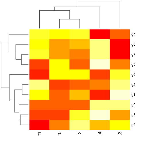
  r.heatmap(mdata)
finally:
  grdevices.dev_off()

Final results:

... and a heatmap plot:

Final note, yes I know there is some fuzz at the bottom of the image with the dendrogram. I don't know why. Maybe someone can fix this ... and yes, that's possible, because all of this is fully open-sourced :-) 

td;dr: https://gist.github.com/4176508