Sage announces 3 GSoC projects

Sage is pleased to announce three Google Summer of Code projects for 2013. They focus on speed improvements of symbolic functions, simplifying the distribution and installation procedure on Debian/Linux and ubiquitous accessibility of Sage on the Android platform.

Mathematical Functions Library

Eviatar Bach –  University of British Columbia in Vancouver, Canada

(Mentor: Flavia Stan, Backup: Burcin Erocal)

Sage interfaces with multiple third-party libraries, such as MPFR, GSL, GP/PARI, mpmath, and Maxima, for numerical evaluation of special functions. There are significant discrepancies between these backends in the performance for numerical approximations of the same expression. An initial benchmark reveals, for example, that calculating spherical_bessel_J(1, 5.2) with SciPy is over 100 times faster than with Maxima.

The project has the following goals:

1. develop a benchmark framework to determine which backend should be used by default to evaluate a special function over a specific domain,
2. create symbolic wrappers for all the special functions that can be evaluated numerically by a package included in Sage,
3. create a data structure for generalized hypergeometric functions and extend the symbolic wrappers to obtain representations in terms of generalized hypergeometric functions when possible,
4. implement closure properties for holonomic functions as a next step to improve the symbolic processing of special functions in Sage.

Overall improvement of the Sage Android application

Rasmi Elasmar

(Mentor: Volker Braun, Backup: Harald Schilly)

Although there are already some existing efforts, Sage is still not easily accessible from the Android platform. The Sage Cell client/server infrastructure is an already existing step towards running Sage on a server and communicating back the results. The aim of this proposal is to fix, improve and update the Sage Android application to include new features and functionality, as well as an improved interface for simpler and improved usability. Android's new "Holo" style, sharing of calculations and results, and much more waits to be realized on Android for Sage.

Get Sage ready for Linux distributions

Felix Salfelder – Goethe Universität, Frankfurt, Germany

(Mentor: Tobias Hansen, Julien Puydt, Jeroen Demeyer & John Palmieri )

sage-devel discussion

The aim of this project is to detach the build process of Sage ("the software") from Sage ("the distribution"). The goal is a build system that works within the context of Sage as well as for any GNU/Linux distribution that ships the dependencies for Sage. Distributions that already ship Sage packages or plan to do so are Fedora and Debian. This project is an important step towards making Sage packages in GNU/Linux distributions feasible.


Sage warmly welcomes all three new students and wishes them all the best to learn something new and make an impact in Sage's future developments!

Sage part of Google's Summer of Code 2013

Good News, like last year Sage is once again part of Google's Summer of Code. This means, until April 22 at 19:00 UTC students can submit their applications and mentors will review them and do the matching.

Please share this with prospective students or think about being a mentor this year!

links:

• Sage's GSoC page
• Ideas (check back for updates)

Sage 5.8

Sage 5.8 has been released, download it here.

Also, the documentation page has been updated to reflect the new thematic tutorials. I highly recommend to browse through all those topics to learn more about Sage's ever increasing scope.

Git, Mercurial, Subversion trends

In case you have to convince someone on which horse to bet:

Lenovo x220 Trackpoint and Ubuntu

Although I'm using my Lenovo x220 laptop for more than a year, I discovered the settings for the track-point yesterday (random searches and forums, don't remember). I was never really thinking about it, but the track-point was a bit slow and stiff. The configuration settings of the usual UI configuration menu had no effect at all (yes, certainly a bug), either.

So, to reveal the magic, here it is. I've added a udev configuration file here:

$ cat /etc/udev/rules.d/trackpoint.rules

SUBSYSTEM=="serio", DRIVERS=="psmouse", WAIT_FOR="/sys/devices/platform/i8042/serio1/serio2/sensitivity", ATTR{sensitivity}="240", ATTR{speed}="95", ATTR{press_to_select}="1", ATTR{inertia}="6"


This is just one line for the settings of sensitivity, speed and intertia. You can also play around with them manually, e.g.

$ echo "5" | sudo tee /sys/devices/platform/i8042/serio1/serio2/inertia

Mathematica 9's R integration vs. Rpy2

Some notes about "What's new in Mathematica 9: Builtin R Integration"
To understand what's going on, please open the example: Hierarchical Clustering.

This posting is basically about how to integrate R via Rpy2 in Python and hence also in Sage.

First thing you should notice is the clash of two parallel worlds. MMA's "RSet" command converts and sets the variable y in the scope of R. That's nice, but wouldn't it be much easier, to just have a local variable for that? Second of all, the function definitions inside strings - filled with escaped quotes - is also not that great. Isn't there are better quoting available?

What I want to do is to accomplish something similar with Rpy2. So yes, there are also equivalents to this RSet function, and you can also evaluate arbitrary R code inside strings (Python has triple-quoting to avoid escaping quotes). But that's not everything. You can import R packages [from rpy2.robjects.packages import importr] and bind them to local variables and have, for example, tab-completion on them. R Functions can be referenced directly, data-sets can be exchanged with implicit converters (e.g. numpy's ndarray -> R's Matrix), etc.

You can see the final output and code here: https://gist.github.com/4176508

Besides the usual import/from stuff common in Python, I start by creating a random matrix with Numpy:


mdata = np.random.randn(10, 5)

Enable autmatic conversion between Numpy and R:


from rpy2.robjects import numpy2ri
numpy2ri.activate()


Print the matrix using R's print:

rprint = robj.globalenv.get("print")
rprint(mdata)

            [,1]        [,2]        [,3]         [,4]        [,5]
 [1,]  2.1844065 -1.05401295  1.18316261 -0.356338229  1.55031790
 [2,]  1.2476473  0.89507075 -0.14576584  0.006899727  0.01350773
 [3,] -1.6416017 -0.28180113  0.02784612  1.199042583  0.01272994
 [4,]  1.8645490  0.30993270  0.18107913  0.131505590  0.57083588
 [5,]  1.2397427  0.73639680 -0.42883124 -0.436741492  0.43644592
 [6,] -0.1980955 -0.04463804 -0.11217381  1.768415923 -1.82884840
 [7,]  0.2943145  2.12648235  0.21068166  1.718289719  0.15711455
 [8,]  0.2453526  0.64922040  1.80518277  0.086208024  1.18789962
 [9,]  0.8229507  0.56227084 -1.72153433 -1.511514201  1.04610492
[10,]  0.1430900  0.03371198 -0.58992825  1.023002088 -1.47153121

... and just for fun, R'summary, printed with Python's print function:

print r.summary(mdata)

         V1                V2                 V3                 V4       
 Min.   :-1.6416   Min.   :-1.05401   Min.   :-1.72153   Min.   :-1.5115
 1st Qu.: 0.1687   1st Qu.:-0.02505   1st Qu.:-0.35806   1st Qu.:-0.2655
 Median : 0.5586   Median : 0.43610   Median :-0.04216   Median : 0.1089
 Mean   : 0.6202   Mean   : 0.39326   Mean   : 0.04097   Mean   : 0.3629
 3rd Qu.: 1.2457   3rd Qu.: 0.71460   3rd Qu.: 0.20328   3rd Qu.: 1.1550
 Max.   : 2.1844   Max.   : 2.12648   Max.   : 1.80518   Max.   : 1.7684
       V5        
 Min.   :-1.82885
 1st Qu.: 0.01292
 Median : 0.29678
 Mean   : 0.16746
 3rd Qu.: 0.92729
 Max.   : 1.55032  

... now applying the labels. This time, I show how to execute R code directly, hence injecting the variable "y" in R's global namespace, too:

from rpy2 import robjects as robj
robj.globalenv['y'] = mdata

r("""
dimnames(y) <- b="b">list(paste("g", 1:10, sep=""),
                    paste("t", 1:5,  sep=""))
y
""")

Compare this to the way you have to do this in MMA9!

--- EDIT
Below is a way how the same is accomplished in Python. The paste command is replaced by Python's list comprehension, the list command is from R and mdata is converted to an R object to be able to do slot assignments.


mdata = numpy2ri.numpy2ri(mdata)
import rpy2.rinterface as ri
descr = ri.baseenv["list"](
         ri.StrSexpVector(['g%s'%_ for _ in range(10)]),
         ri.StrSexpVector(['t%s'%_ for _ in range(5)]))
mdata.do_slot_assign("dimnames", descr)

The first example is certainly more pleaseant, but once you would create some neat aliases for the R functions (e.g. list = ri.baseenv["list"]; strv = ri.StrSexpVector; ...), working in Python shouldn't be hard, too.
--- END EDIT

Calculating the correlation and distance matrix. Notice, that dots in R's functions, like the as.dist(), are converted to underscores in Python. Those dots are just like normal letters in the identifier name, nothing further.

stats = importr("stats")

corrm = r.cor(r.t(mdata), method="spearman")
# no idea how to do 1-matrix automagically
robj.globalenv['corrm'] = corrm
distm = stats.as_dist(r("1-corrm"))

rprint(corrm)
rprint(distm)

      [,1] [,2] [,3] [,4] [,5] [,6] [,7] [,8] [,9] [,10]
 [1,]  1.0 -0.3  0.1  0.5 -0.2  0.9  0.8  0.6  0.3   0.2
 [2,] -0.3  1.0  0.6  0.3  0.7 -0.4  0.0  0.1  0.2  -0.5
 [3,]  0.1  0.6  1.0 -0.1 -0.1 -0.3 -0.1  0.7  0.6  -0.9
 [4,]  0.5  0.3 -0.1  1.0  0.7  0.6  0.7 -0.1 -0.3   0.3
 [5,] -0.2  0.7 -0.1  0.7  1.0  0.0  0.3 -0.4 -0.3   0.2
 [6,]  0.9 -0.4 -0.3  0.6  0.0  1.0  0.9  0.3  0.1   0.6
 [7,]  0.8  0.0 -0.1  0.7  0.3  0.9  1.0  0.4  0.3   0.5
 [8,]  0.6  0.1  0.7 -0.1 -0.4  0.3  0.4  1.0  0.9  -0.4
 [9,]  0.3  0.2  0.6 -0.3 -0.3  0.1  0.3  0.9  1.0  -0.3
[10,]  0.2 -0.5 -0.9  0.3  0.2  0.6  0.5 -0.4 -0.3   1.0


 
     1   2   3   4   5   6   7   8   9
2  1.3                               
3  0.9 0.4                           
4  0.5 0.7 1.1                       
5  1.2 0.3 1.1 0.3                   
6  0.1 1.4 1.3 0.4 1.0               
7  0.2 1.0 1.1 0.3 0.7 0.1           
8  0.4 0.9 0.3 1.1 1.4 0.7 0.6       
9  0.7 0.8 0.4 1.3 1.3 0.9 0.7 0.1   
10 0.8 1.5 1.9 0.7 0.8 0.4 0.5 1.4 1.3


The clustering happens below (note: I had to execute the "NULL" in the r context, because it seems that Python's "None" isn't converted)

hr = stats.hclust(distm, method = "complete", members = r("NULL"))

Plotting is straightforward too. To plot to a device besides X11, one has to be a bit more specific. The documentation is full of examples. Notice, the only special part is the mfrow=r.c(1,2). 

Looking at Wolfram's blogpost, I really don't want to understand what MMA's "getRPlot[...]" calling "mathematicaRPlotWrapper" does.

grdevices = importr('grDevices')
grdevices.png(file="mma9rpy2.png", width=512, height=300)
try:
  r.par(mfrow = r.c(1,2))
  r.plot(hr, hang = 0.1)
  r.plot(hr, hang = -0.1)
finally:
  grdevices.dev_off()

grdevices.png(file="mma9rpy2-2.png", width = 512, height = 512)
try:
  r.heatmap(mdata)
finally:
  grdevices.dev_off()

Final results:

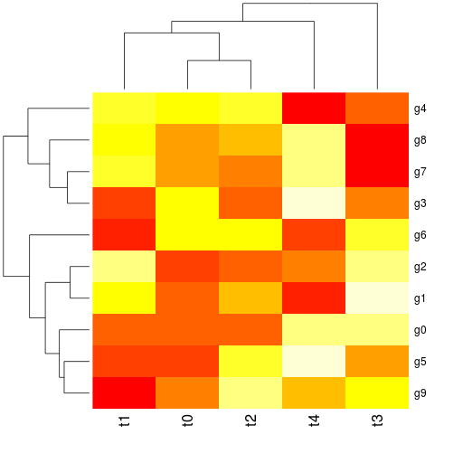
... and a heatmap plot:

Final note, yes I know there is some fuzz at the bottom of the image with the dendrogram. I don't know why. Maybe someone can fix this ... and yes, that's possible, because all of this is fully open-sourced :-) 

td;dr: https://gist.github.com/4176508

Sage 5.4.1 Released

Sage 5.4.1 was released on 15 November 2012. 

It is available in source and binary form from:

• http://www.sagemath.org/download.html
• http://www.sagemath.org/mirror/torrents.html

Sage (http://www.sagemath.org/) is developed by volunteers and combines over 90 open source packages. For instructions about installing Sage, see

•  http://www.sagemath.org/doc/installation

The following page lists the platforms on which Sage should work:

•   http://wiki.sagemath.org/SupportedPlatforms

If you have any questions and/or problems, please report them to any of these Google groups:

•   sage-support: http://groups.google.com/group/sage-support
•   sage-devel: http://groups.google.com/group/sage-devel

You can also drop by in #sagemath on freenode or post your questions at http://ask.sagemath.org/

The following 15 people contributed to this release. Of those, 2 made their first contribution to Sage:

  - Aly Deines
  - Benjamin Hutz [first contribution]
  - Burcin Erocal
  - David Loeffler
  - Dmitrii Pasechnik
  - Jeroen Demeyer
  - John Palmieri
  - Karl-Dieter Crisman
  - Kenneth Smith
  - Paul Zimmermann
  - Punarbasu Purkayastha
  - Sarah Chisholm
  - Sebastien Gouezel [first contribution]
  - Travis Scrimshaw
  - Volker Braun

* Release manager: Jeroen Demeyer.

* We closed 13 tickets in this release. For details, see

  http://boxen.math.washington.edu/home/release/sage-5.4.1/tickets.html

Closed tickets:

#13309: Build Sage on OS X Mountain Lion [Reviewed by Dmitrii Pasechnik]

Merged in sage-5.4.1.rc0:

#6367: Karl-Dieter Crisman, Kenneth Smith: polygon2d -- several issues: typo in docs, shouldn't have been renamed [Reviewed by Volker Braun]
#10803: Paul Zimmermann: critical bug in real_roots [Reviewed by Jeroen Demeyer]
#12753: Benjamin Hutz: is_PrimeField import error [Reviewed by David Loeffler]
#12859: Aly Deines: quaternion algebra 'ramified at one prime' [Reviewed by Sarah Chisholm]
#13382: Dmitrii Pasechnik: build docs for SymmetricGroupRepresentation(s) [Reviewed by Volker Braun, Travis Scrimshaw]

#13533: Jeroen Demeyer: Remove "optional - gcc" from doctests [Reviewed
by Karl-Dieter Crisman, John Palmieri]
#13541: John Palmieri: update scipy to 0.11.0 [Reviewed by Dmitrii Pasechnik]
#13598: John Palmieri: 'x' should be defined when using 'sage -c' [Reviewed by Punarbasu Purkayastha]
#13632: Sebastien Gouezel: Fix latex display of arguments of symbolic functions [Reviewed by Burcin Erocal] 

Merged in sage-5.4.1.rc1:

#13407: Jeroen Demeyer: Move sage-make_relative to sage-location [Reviewed by Dmitrii Pasechnik]
#13452: Jeroen Demeyer: Refactor sage-location [Reviewed by Dmitrii Pasechnik]
#13689: Jeroen Demeyer: Fix upgrading from relocated Sage with GCC [Reviewed by John Palmieri]